Query Tuning
On this page
Things to Consider Before Query Tuning
Before creating your database, it's important to consider the workload that will be placed upon it.
Concurrency is the number of queries that are executing a on the database the same time.
Throughput is the number of queries that are executing per unit of time.
Latency is the query execution time.
Lastly, your cluster size will determine the throughput and performance of databases in the cluster.
You can utilize Use the Workload Manager and Set Resource Limits as tools to manage cluster workload and define resource pools that can improve query performance.
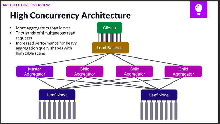
Tradeoff between Aggregator Count and Leaf Count
When high concurrency is of the utmost importance, it is best to have more aggregator nodes than leaf nodes since the aggregator receives data requests from users.
Conversely, if low latency is more important than high concurrently, then it is better to have more leaf nodes (and therefore, more partitions) since the data is stored on leaf nodes.
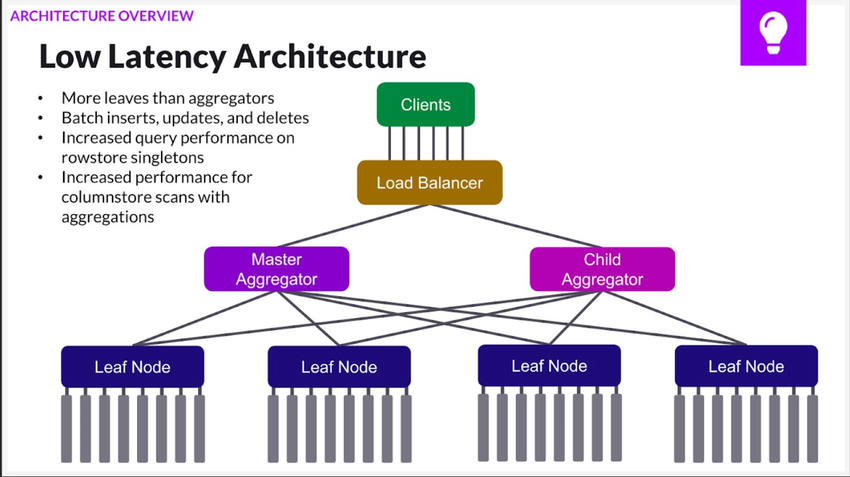
To adjust your aggregators and leaf node counts, please see the Cluster Management Commands page.
Run ANALYZE
The ANALYZE command collects data statistics on a table to facilitate accurate query optimization.ANALYZE your tables after inserting, updating, or deleting large numbers of rows (30% of your table row count is a good rule of thumb).
Look for Hot Queries
You can do query analysis on hot running queries by using the Workload Monitoring and SingleStore Visual Explain features, or by running the SHOW PLANCACHE command.
For example, you can use a query like the following to see the select queries with the highest average execution time.
SELECT Database_Name, Query_Text, Commits, Execution_Time, Execution_Time/Commits AS avg_time_ms, Average_Memory_UseFROM information_schema.plancacheWHERE Query_Text LIKE 'select%'ORDER BY avg_time_ms DESC;
Check if Queries are Using Indexes
One important query performance consideration is adding appropriate indexes for your queries.
Indexes for Filters
Consider the following rowstore table:
CREATE ROWSTORE TABLE qtune_1 (a INT, b INT);
Suppose we are running queries like:
SELECT * FROM qtune_1 WHERE a = 3;
EXPLAIN shows that running the query against the current table schema requires a full TableScan - scanning all the rows of t, which is unnecessarily expensive if a small fraction of the values in t equal 3.
EXPLAIN SELECT * FROM qtune_1 WHERE a = 3;
+------------------------------------------------------------------+
| EXPLAIN                                                          |
+------------------------------------------------------------------+
| Gather partitions:all alias:remote_0 parallelism_level:partition |
| Project [qtune_1.a, qtune_1.b]                                   |
| Filter [qtune_1.a = 3]                                           |
| TableScan test1.qtune_1 table_type:sharded_rowstore              |
+------------------------------------------------------------------+
If an index is added, the query will instead use an IndexRangeScan on the key a:
ALTER TABLE qtune_1 ADD INDEX (a);EXPLAIN SELECT * FROM qtune_1 WHERE a = 3;
+----------------------------------------------------------------------------------+
| EXPLAIN                                                                          |
+----------------------------------------------------------------------------------+
| Gather partitions:all alias:remote_0 parallelism_level:partition                 |
| Project [qtune_1.a, qtune_1.b]                                                   |
| IndexRangeScan test1.qtune_1, KEY a (a) scan:[a = 3] table_type:sharded_rowstore |
+----------------------------------------------------------------------------------+
A query that filters on both a and b is unable to take advantage of the filtering on b to reduce the rows that need to be scanned.a = 3 only.
EXPLAIN SELECT * FROM qtune_1 WHERE a = 3 AND b = 4;
+----------------------------------------------------------------------------------+
| EXPLAIN                                                                          |
+----------------------------------------------------------------------------------+
| Gather partitions:all alias:remote_0 parallelism_level:partition                 |
| Project [qtune_1.a, qtune_1.b]                                                   |
| Filter [qtune_1.b = 4]                                                           |
| IndexRangeScan test1.qtune_1, KEY a (a) scan:[a = 3] table_type:sharded_rowstore |
+----------------------------------------------------------------------------------+
Adding an index on b allows the query to scan more selectively:
ALTER TABLE qtune_1 ADD INDEX (b);EXPLAIN SELECT * FROM qtune_1 WHERE a = 3 AND b = 4;
+-------------------------------------------------------------------------------------------------+
| EXPLAIN                                                                                         |
+-------------------------------------------------------------------------------------------------+
| Gather partitions:all alias:remote_0 parallelism_level:partition                                |
| Project [qtune_1.a, qtune_1.b]                                                                  |
| IndexRangeScan test1.qtune_1, KEY a_2 (a, b) scan:[a = 3 AND b = 4] table_type:sharded_rowstore |
+-------------------------------------------------------------------------------------------------+
For columnstore tables, it's a best practice to set a sort key the table to take advantage of segment elimination.
Segment elimination occurs when filtering on the sort key.
Consider a columnstore table with an explicit sort key:
CREATE TABLE qtune_2 (a int, b int, SORT KEY(a));
Suppose the following queries are run:
SELECT * FROM qtune_2 WHERE a = 3;
EXPLAIN shows that running the query against this table schema requires a ColumnStoreScan - scanning the segments (column a) which contain values equal to 3.3 are not scanned.3:
EXPLAIN SELECT * FROM qtune_2 WHERE a = 3;
+------------------------------------------------------------------------------+
| EXPLAIN                                                                      |
+------------------------------------------------------------------------------+
| Gather partitions:all alias:remote_0 parallelism_level:segment               |
| Project [qtune_2.a, qtune_2.b]                                               |
| ColumnStoreFilter [qtune_2.a = 3]                                            |
| ColumnStoreScan test1.qtune_2, SORT KEY a (a) table_type:sharded_columnstore |
+------------------------------------------------------------------------------+
Indexes for GROUP BY and ORDER BY
Another class of cases where indexes can improve query performance is GROUP BY and ORDER BY .
Consider this rowstore table:
CREATE ROWSTORE TABLE qtune_3 (a int, b int);
Executing the following query requires a HashGroupBy.a:
EXPLAIN SELECT a, SUM(b) FROM qtune_3 GROUP BY a;
+-------------------------------------------------------------------------------------+
| EXPLAIN                                                                             |
+-------------------------------------------------------------------------------------+
| Project [remote_0.a, `SUM(b)`] est_rows:1                                           |
| HashGroupBy [SUM(remote_0.`SUM(b)`) AS `SUM(b)`] groups:[remote_0.a]                |
| Gather partitions:all est_rows:1 alias:remote_0 parallelism_level:partition         |
| Project [qtune_3.a, `SUM(b)`] est_rows:1                                            |
| HashGroupBy [SUM(qtune_3.b) AS `SUM(b)`] groups:[qtune_3.a]                         |
| TableScan test1.qtune_3 table_type:sharded_rowstore est_table_rows:1 est_filtered:1 |
+-------------------------------------------------------------------------------------+
However, with an index on a, SingleStore can execute the query with a StreamingGroupBy operation because by scanning the index on a, it can process all elements of a group consecutively.
ALTER TABLE qtune_3 ADD INDEX(a);EXPLAIN SELECT a, SUM(b) FROM qtune_3 GROUP BY a;
+------------------------------------------------------------------------------------------------+
| EXPLAIN                                                                                        |
+------------------------------------------------------------------------------------------------+
| Project [remote_0.a] est_rows:1                                                                |
| HashGroupBy [] groups:[remote_0.a]                                                             |
| Gather partitions:all est_rows:1 alias:remote_0 parallelism_level:partition                    |
| Project [qtune_3.a] est_rows:1                                                                 |
| StreamingGroupBy [] groups:[qtune_3.a]                                                         |
| TableScan test1.qtune_3, KEY a (a) table_type:sharded_rowstore est_table_rows:1 est_filtered:1 |
+------------------------------------------------------------------------------------------------+
For a columnstore table, the column(s) in the GROUP BY clause must match the SORT KEY for a StreamingGroupBy to be considered.
An ORDER BY on a rowstore table without an index, SingleStore needs to sort:
CREATE ROWSTORE TABLE qtune_4 (a INT, b INT);
EXPLAIN SELECT * FROM qtune_4 ORDER BY b;
+------------------------------------------------------------------+
| EXPLAIN                                                          |
+------------------------------------------------------------------+
| Project [remote_0.a, remote_0.b]                                 |
| Sort [remote_0.b]                                                |
| Gather partitions:all alias:remote_0 parallelism_level:partition |
| Project [qtune_4.a, qtune_4.b]                                   |
| Sort [qtune_4.b]                                                 |
| TableScan test1.qtune_4 table_type:sharded_rowstore              |
+------------------------------------------------------------------+
With an index, SingleStore can eliminate the need to sort:
ALTER TABLE qtune_4 ADD INDEX (b);EXPLAIN SELECT * FROM qtune_4 ORDER BY b;
+----------------------------------------+
| EXPLAIN                                |
+----------------------------------------+
| Project [qtune_4.a, qtune_4.b]         |
| GatherMerge [qtune_4.b] partitions:all |
| Project [qtune_4.a, qtune_4.b]         |
| TableScan test1.qtune_4, KEY b (b)     |
+----------------------------------------+
As mentioned above, it's a best practice to set a sort key on columnstore tables to take advantage of segment elimination on queries with GROUP BY and ORDER BY clauses.
Fanout vs Single-Partition Queries
SingleStore’s distributed architecture takes advantage of CPUs from many servers to execute your queries.
Using this table as an example:
CREATE TABLE urls (domain varchar(128),path varchar(8192),time_sec int,status_code binary(3),...shard key (domain, path, time_sec));
The following query only involves a single partition because it has equality filters on all columns of the shard key, so the rows which match can only be on a single partition.EXPLAIN, Gather partitions:single indicates SingleStore is using a single-partition plan.
EXPLAIN SELECT status_code FROM urlsWHERE domain = 'youtube.com' AND path = '/watch?v=euh_uqxwk58' AND time_sec = 1;
+-------------------------------------------------------------------------------------------------------------------------------------------------------+
| EXPLAIN                                                                                                                                               |
+-------------------------------------------------------------------------------------------------------------------------------------------------------+
| Gather partitions:single                                                                                                                              |
| Project [urls.status_code]                                                                                                                            |
| IndexRangeScan test2.urls, SHARD KEY domain (domain, path, time_sec) scan:[domain = "youtube.com" AND path = "/watch?v=euh_uqxwk58" AND time_sec = 1] |
+-------------------------------------------------------------------------------------------------------------------------------------------------------+
The following query which does not filter on time_, does not match a single partition.Gather partitions:all.
EXPLAIN SELECT status_code FROM urlsWHERE domain = 'youtube.com'AND path = '/watch?v=euh_uqxwk58';
+--------------------------------------------------------------------------------------------------------------------------------------+
| EXPLAIN                                                                                                                              |
+--------------------------------------------------------------------------------------------------------------------------------------+
| Project [urls.status_code]                                                                                                           |
| Gather partitions:all                                                                                                                |
| Project [urls.status_code]                                                                                                           |
| IndexRangeScan test2.urls, SHARD KEY domain (domain, path, time_sec) scan:[domain = "youtube.com" AND path = "/watch?v=euh_uqxwk58"] |
+--------------------------------------------------------------------------------------------------------------------------------------
To fix this, the table urls could be sharded on domain.(domain,path).
Distributed Joins
SingleStore’s query execution architecture allows you to run arbitrary SQL queries on any table regardless of data distribution.
Collocating Joins
Consider the following tables:
CREATE TABLE lineitem(l_orderkey INT NOT NULL,l_linenumber INT NOT NULL,...PRIMARY KEY(l_orderkey, l_linenumber));
CREATE TABLE orders(o_orderkey INT NOT NULL,...PRIMARY KEY(o_orderkey));
When lineitem and orders are joined with the current schema, a distributed join is performed and data is repartitioned from the lineitem table.
EXPLAIN SELECT COUNT(*) FROM lineitemJOIN orders ON o_orderkey = l_orderkey;
+---------------------------------------------------------------------------------------------------------------------------------+
| EXPLAIN                                                                                                                         |
+---------------------------------------------------------------------------------------------------------------------------------+
| Project [`COUNT(*)`]                                                                                                            |
| Aggregate [SUM(`COUNT(*)`) AS `COUNT(*)`]                                                                                       |
| Gather partitions:all est_rows:1                                                                                                |
| Project [`COUNT(*)`] est_rows:1 est_select_cost:1762812                                                                         |
| Aggregate [COUNT(*) AS `COUNT(*)`]                                                                                              |
| NestedLoopJoin                                                                                                                  |
| |---IndexSeek test.orders, PRIMARY KEY (o_orderkey) scan:[o_orderkey = r0.l_orderkey] est_table_rows:565020 est_filtered:565020 |
| TableScan r0 storage:list stream:no                                                                                             |
| Repartition [lineitem.l_orderkey] AS r0 shard_key:[l_orderkey] est_rows:587604                                                  |
| TableScan test.lineitem, PRIMARY KEY (l_orderkey, l_linenumber) est_table_rows:587604 est_filtered:587604                       |
+---------------------------------------------------------------------------------------------------------------------------------+
The performance of this query can be improved by adding an explicit shard key to the lineitemtable on l_.lineitem and orders.
+--------------------------------------------------------------------------------------------------------------------+| EXPLAIN |+--------------------------------------------------------------------------------------------------------------------+| Project [`COUNT(*)`] || Aggregate [SUM(`COUNT(*)`) AS `COUNT(*)`] || Gather partitions:all || Project [`COUNT(*)`] || Aggregate [COUNT(*) AS `COUNT(*)`] || ChoosePlan || | :estimate || | SELECT COUNT(*) AS cost FROM test.lineitem || | SELECT COUNT(*) AS cost FROM test.orders || |---NestedLoopJoin || | |---IndexSeek test.orders, PRIMARY KEY (o_orderkey) scan:[o_orderkey = lineitem.l_orderkey] || | TableScan test.lineitem, PRIMARY KEY (l_orderkey, l_linenumber) || +---NestedLoopJoin || |---IndexRangeScan test.lineitem, PRIMARY KEY (l_orderkey, l_linenumber) scan:[l_orderkey = orders.o_orderkey] || TableScan test.orders, PRIMARY KEY (o_orderkey) |+--------------------------------------------------------------------------------------------------------------------+
Reference Table Joins
Reference tables are replicated to each aggregator and leaf in the cluster, therefore their use case is best for data that is small and slowly changing.
Consider the following schema:
CREATE TABLE customer(c_custkey INT NOT NULL,c_nationkey INT NOT NULL,...PRIMARY KEY(c_custkey),key(c_nationkey));
CREATE TABLE nation(n_nationkey INT NOT NULL,...PRIMARY KEY(n_nationkey));
With the current schema, when we join the customer and nation tables together on nationkey, the nation table must be broadcast each time the query is run.
EXPLAIN SELECT COUNT(*) FROM customerJOIN nation ON n_nationkey = c_nationkey;
+-------------------------------------------------------------------------------------------------------------------------------------------------+
| EXPLAIN                                                                                                                                         |
+-------------------------------------------------------------------------------------------------------------------------------------------------+
| Project [`Count(*)`]                                                                                                                            |
| Aggregate [SUM(`Count(*)`) AS `Count(*)`]                                                                                                       |
| Gather partitions:all est_rows:1                                                                                                                |
| Project [`Count(*)`] est_rows:1 est_select_cost:1860408                                                                                         |
| Aggregate [COUNT(*) AS `Count(*)`]                                                                                                              |
| NestedLoopJoin                                                                                                                                  |
| |---IndexRangeScan test.customer, KEY c_nationkey (c_nationkey) scan:[c_nationkey = r1.n_nationkey] est_table_rows:1856808 est_filtered:1856808 |
| TableScan r1 storage:list stream:no                                                                                                             |
| Broadcast [nation.n_nationkey] AS r1 est_rows:300                                                                                               |
| TableScan test.nation, PRIMARY KEY (n_nationkey) est_table_rows:300 est_filtered:300                                                            |
+-------------------------------------------------------------------------------------------------------------------------------------------------+
The broadcast can be avoided by making nation a reference table as it is relatively small and changes rarely.
CREATE REFERENCE TABLE nation(n_nationkey INT NOT NULL,...PRIMARY KEY(n_nationkey));
EXPLAIN SELECT COUNT(*) FROM customerJOIN nation ON n_nationkey = c_nationkey;
+-------------------------------------------------------------------------------------------------------------+
| EXPLAIN                                                                                                     |
+-------------------------------------------------------------------------------------------------------------+
| Project [`Count(*)`]                                                                                        |
| Aggregate [SUM(`Count(*)`) AS `Count(*)`]                                                                   |
| Gather partitions:all                                                                                       |
| Project [`Count(*)`]                                                                                        |
| Aggregate [COUNT(*) AS `Count(*)`]                                                                          |
| ChoosePlan                                                                                                  |
| |   :estimate                                                                                               |
| |       SELECT COUNT(*) AS cost FROM test.customer                                                          |
| |       SELECT COUNT(*) AS cost FROM test.nation                                                            |
| |---NestedLoopJoin                                                                                          |
| |   |---IndexSeek test.nation, PRIMARY KEY (n_nationkey) scan:[n_nationkey = customer.c_nationkey]          |
| |   TableScan test.customer, PRIMARY KEY (c_custkey)                                                        |
| +---NestedLoopJoin                                                                                          |
|     |---IndexRangeScan test.customer, KEY c_nationkey (c_nationkey) scan:[c_nationkey = nation.n_nationkey] |
|     TableScan test.nation, PRIMARY KEY (n_nationkey)                                                        |
+-------------------------------------------------------------------------------------------------------------+
Joins on the Aggregator
Consider the following schema and row counts:
CREATE TABLE customer(c_custkey INT NOT NULL,c_acctbal DECIMAL(15,2) NOT NULL,PRIMARY KEY(c_custkey));
CREATE TABLE orders(o_orderkey INT NOT NULL,o_custkey INT NOT NULL,o_orderstatus varchar(20) NOT NULL,PRIMARY KEY(o_orderkey),key(o_custkey));
SELECT COUNT(*) FROM orders;
+----------+
| COUNT(*) |
+----------+
|   429786 |
+----------+SELECT COUNT(*) FROM orders WHERE o_orderstatus = 'open';
+----------+
| COUNT(*) |
+----------+
|     1000 |
+----------+SELECT COUNT(*) FROM orders WHERE o_orderstatus = 'open';
+----------+
| COUNT(*) |
+----------+
|     1000 |
+----------+SELECT COUNT(*) FROM customer;
+----------+
| COUNT(*) |
+----------+
|  1014726 |
+----------+SELECT COUNT(*) FROM customer WHERE c_acctbal > 100.0;
+----------+
| COUNT(*) |
+----------+
|      988 |
+----------+
Note that while customer and orders are fairly large, when a query is filtered on open orders and account balances greater than 100, relatively few rows match.orders and customer are joined using these filters, the join can be performed on an aggregator.EXPLAIN as having a separate Gather operator for orders and customer and a HashJoin operator above the Gather .
EXPLAIN SELECT o_orderkey FROM customerJOIN ordersWHERE c_acctbal > 100.0 AND o_orderstatus = 'open' AND o_custkey = c_custkey;
+------------------------------------------------------------------+
| EXPLAIN                                                          |
+------------------------------------------------------------------+
| Project [orders.o_orderkey]                                      |
| HashJoin [orders.o_custkey = customer.c_custkey]                 |
| |---TempTable                                                    |
| |   Gather partitions:all                                        |
| |   Project [orders_0.o_orderkey, orders_0.o_custkey]            |
| |   Filter [orders_0.o_orderstatus = "open"]                     |
| |   TableScan test3.orders AS orders_0, PRIMARY KEY (o_orderkey) |
| TableScan 0tmp AS customer storage:list stream:yes               |
| TempTable                                                        |
| Gather partitions:all                                            |
| Project [customer_0.c_custkey]                                   |
| Filter [customer_0.c_acctbal > 100.0]                            |
| TableScan test3.customer AS customer_0, PRIMARY KEY (c_custkey)  |
+------------------------------------------------------------------+
By default, SingleStore will perform this optimization when each Gather pulls less than 120,000 rows from the leaves.max_ variable.leaf_ hint.leaf_ hint forces the optimizer to perform as much work as possible on the leaf nodes.
EXPLAIN SELECT WITH(LEAF_PUSHDOWN=TRUE) o_orderkey FROM customerJOIN ordersWHERE c_acctbal > 100.0 AND o_orderstatus = 'open' AND o_custkey = c_custkey;
+--------------------------------------------------------------------------------------------------------------------------------+
| EXPLAIN                                                                                                                        |
+--------------------------------------------------------------------------------------------------------------------------------+
| Project [r0.o_orderkey]                                                                                                        |
| Gather partitions:all est_rows:11                                                                                              |
| Project [r0.o_orderkey] est_rows:11 est_select_cost:1955                                                                       |
| Filter [customer.c_acctbal > 100.0]                                                                                            |
| NestedLoopJoin                                                                                                                 |
| |---IndexSeek test3.customer, PRIMARY KEY (c_custkey) scan:[c_custkey = r0.o_custkey] est_table_rows:1013436 est_filtered:1092 |
| TableScan r0 storage:list stream:no                                                                                            |
| Repartition [orders.o_orderkey, orders.o_custkey] AS r0 shard_key:[o_custkey] est_rows:972                                     |
| Filter [orders.o_orderstatus = "open"]                                                                                         |
| TableScan test3.orders, PRIMARY KEY (o_orderkey) est_table_rows:92628 est_filtered:972                                         |
+--------------------------------------------------------------------------------------------------------------------------------+SET max_subselect_aggregator_rowcount=500;
EXPLAIN SELECT o_orderkey FROM customerJOIN ordersWHERE c_acctbal > 100.0 AND o_orderstatus = 'open' AND o_custkey = c_custkey;
+--------------------------------------------------------------------------------------------------------------------------------+
| EXPLAIN                                                                                                                        |
+--------------------------------------------------------------------------------------------------------------------------------+
| Project [r0.o_orderkey]                                                                                                        |
| Gather partitions:all est_rows:11                                                                                              |
| Project [r0.o_orderkey] est_rows:11 est_select_cost:1955                                                                       |
| Filter [customer.c_acctbal > 100.0]                                                                                            |
| NestedLoopJoin                                                                                                                 |
| |---IndexSeek test3.customer, PRIMARY KEY (c_custkey) scan:[c_custkey = r0.o_custkey] est_table_rows:1013436 est_filtered:1092 |
| TableScan r0 storage:list stream:no                                                                                            |
| Repartition [orders.o_orderkey, orders.o_custkey] AS r0 shard_key:[o_custkey] est_rows:972                                     |
| Filter [orders.o_orderstatus = "open"]                                                                                         |
| TableScan test3.orders, PRIMARY KEY (o_orderkey) est_table_rows:92628 est_filtered:972                                         |
+--------------------------------------------------------------------------------------------------------------------------------+
Managing Concurrency for Distributed Joins
Queries that require cross-shard data movement, i.
In most scenarios, the default settings for workload management will schedule your workload appropriately to utilize cluster resources without exhausting connection and thread limits.
Related Topics
-
Training: Query Tuning
-
Training: Performance Benchmarking
In this section
Last modified: May 7, 2024